TIP

本文主要是介绍 Sklearn-简单实战案例 。

• 使用python机器学习六（scikit-learn实战）
• 数据加载
• 数据标准化
• 特征的选取
• 算法的开发
  • 逻辑回归
  • 朴素贝叶斯
  • k-最近邻
  • 决策树
  • 支持向量机
• 如何优化算法的参数
• 参考
• 参考文章

使用python机器学习六（scikit-learn实战）

数据加载

首先，数据要被加载到内存中，才能对其操作。Scikit-Learn库在它的实现中使用了NumPy数组，所以我们将用Numpy来加载*.csv文件。让我们从UCI Machine Learning Repository (opens new window)下载其中印度人糖尿病的数据集。 该数据集共有九列，分别为:

怀孕次数 口服葡萄糖耐量试验中2小时中血浆葡萄糖浓度 舒张压（mm Hg） 三头肌皮褶厚度（mm） 2小时血清胰岛素（μU/ ml） 体重指数（kg /（身高（m））^ 2） 糖尿病谱系功能 年龄 是否得糖尿病label

import numpy as np
import urllib.request
# url with dataset
url = "http://archive.ics.uci.edu/ml/machine-learning-databases/pima-indians-diabetes/pima-indians-diabetes.data"
# download the file
raw_data = urllib.request.urlopen(url)
# load the CSV file as a numpy matrix
dataset = np.loadtxt(raw_data, delimiter=",")
# separate the data from the target attributes
X = dataset[:,0:8]
y = dataset[:,8]
print("size:",dataset.size)

X作为特征向量，y作为目标变量。

数据标准化

我们都知道大多数的梯度方法（几乎所有的机器学习算法都基于此）对于数据的缩放很敏感。因此，在运行算法之前，我们应该进行标准化、规格化（归一化）。标准化是将数据按比例缩放，使之落入一个小的特定区间。 归一化是一种简化计算的方式，即将有量纲的表达式，经过变换，化为无量纲的表达式，成为纯量，把数据映射到0～1范围之内处理。Scikit-Learn库已经为其提供了相应的函数。

from sklearn import preprocessing
# standardize the data attributes
standardized_X = preprocessing.scale(X)
# normalize the data attributes
normalized_X = preprocessing.normalize(X)

特征的选取

毫无疑问，解决一个问题最重要的是恰当选取特征、甚至创造特征的能力。这叫做特征选取和特征工程。虽然特征工程是一个相当有创造性的过程，有时候更多的是靠直觉和专业的知识，但对于特征的选取，已经有很多的算法可供直接使用。如树算法就可以计算特征的信息量。

from sklearn import metrics
from sklearn.ensemble import ExtraTreesClassifier
model = ExtraTreesClassifier()
model.fit(X, y)
# display the relative importance of each attribute
print(model.feature_importances_)

output:

[ 0.11193263  0.26076795  0.10153987  0.08278266  0.07190955  0.12292174   0.11527441  0.13287119]

其他所有的方法都是基于对特征子集的高效搜索，从而找到最好的子集，意味着演化了的模型在这个子集上有最好的质量。递归特征消除算法（RFE）是这些搜索算法的其中之一，Scikit-Learn库同样也有提供。

from sklearn.feature_selection import RFE
from sklearn.linear_model import LogisticRegression
model = LogisticRegression()
# create the RFE model and select 3 attributes
rfe = RFE(model, 3)
rfe = rfe.fit(X, y)
# summarize the selection of the attributes
print(rfe.support_)
print(rfe.ranking_)

output

[ True False False False False  True  True False]
[1 2 3 5 6 1 1 4]

算法的开发

正像我说的，Scikit-Learn库已经实现了所有基本机器学习的算法。让我们来瞧一瞧它们中的一些。

逻辑回归

大多数情况下被用来解决分类问题（二元分类），但多类的分类（所谓的一对多方法）也适用。这个算法的优点是对于每一个输出的对象都有一个对应类别的概率。

from sklearn import metrics
from sklearn.linear_model import LogisticRegression
model = LogisticRegression()
model.fit(X, y)
print(model)
# make predictions
expected = y
predicted = model.predict(X)
# summarize the fit of the model
print(metrics.classification_report(expected, predicted))
print(metrics.confusion_matrix(expected, predicted))

output

LogisticRegression(C=1.0, class_weight=None, dual=False, fit_intercept=True,
          intercept_scaling=1, max_iter=100, multi_class='ovr', n_jobs=1,
          penalty='l2', random_state=None, solver='liblinear', tol=0.0001,
          verbose=0, warm_start=False)
             precision    recall  f1-score   support

        0.0       0.79      0.90      0.84       500
        1.0       0.74      0.55      0.63       268

avg / total       0.77      0.77      0.77       768

[[448  52]
 [121 147]]

准确率(accuracy),其定义是: 对于给定的测试数据集，分类器正确分类的样本数与总样本数之比。 精确率(precision)计算的是所有"正确被检索的item(TP)"占所有"实际被检索到的(TP+FP)"的比例.

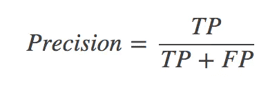
precision

召回率(recall)计算的是所有"正确被检索的item(TP)"占所有"应该检索到的item(TP+FN)"的比例。

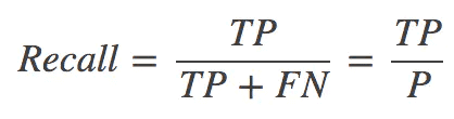
recall

F1-score

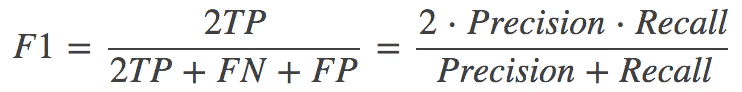
F1-score

可以看到，recall 体现了分类模型H对正样本的识别能力，recall 越高，说明模型对正样本的识别能力越强，precision 体现了模型对负样本的区分能力，precision越高，说明模型对负样本的区分能力越强。F1-score 是两者的综合。F1-score 越高，说明分类模型越稳健。

朴素贝叶斯

它也是最有名的机器学习的算法之一，它的主要任务是恢复训练样本的数据分布密度。这个方法通常在多类的分类问题上表现的很好。

from sklearn import metrics
from sklearn.naive_bayes import GaussianNB
model = GaussianNB()
model.fit(X, y)
print(model)
# make predictions
expected = y
predicted = model.predict(X)
# summarize the fit of the model
print(metrics.classification_report(expected, predicted))
print(metrics.confusion_matrix(expected, predicted))

output

GaussianNB(priors=None)
             precision    recall  f1-score   support

        0.0       0.80      0.84      0.82       500
        1.0       0.68      0.62      0.64       268

avg / total       0.76      0.76      0.76       768

[[421  79]
 [103 165]]

k-最近邻

kNN（k-最近邻）方法通常用于一个更复杂分类算法的一部分。例如，我们可以用它的估计值做为一个对象的特征。有时候，一个简单的kNN算法在良好选择的特征上会有很出色的表现。当参数（主要是metrics）被设置得当，这个算法在回归问题中通常表现出最好的质量。

from sklearn import metrics
from sklearn.neighbors import KNeighborsClassifier
# fit a k-nearest neighbor model to the data
model = KNeighborsClassifier()
model.fit(X, y)
print(model)
# make predictions
expected = y
predicted = model.predict(X)
# summarize the fit of the model
print(metrics.classification_report(expected, predicted))
print(metrics.confusion_matrix(expected, predicted))

output

KNeighborsClassifier(algorithm='auto', leaf_size=30, metric='minkowski',
           metric_params=None, n_jobs=1, n_neighbors=5, p=2,
           weights='uniform')
             precision    recall  f1-score   support

        0.0       0.83      0.88      0.85       500
        1.0       0.75      0.65      0.70       268

avg / total       0.80      0.80      0.80       768

[[442  58]
 [ 93 175]]

决策树

分类和回归树（CART）经常被用于这么一类问题，在这类问题中对象有可分类的特征且被用于回归和分类问题。决策树很适用于多类分类。

from sklearn import metrics
from sklearn.tree import DecisionTreeClassifier
# fit a CART model to the data
model = DecisionTreeClassifier()
model.fit(X, y)
print(model)
# make predictions
expected = y
predicted = model.predict(X)
# summarize the fit of the model
print(metrics.classification_report(expected, predicted))
print(metrics.confusion_matrix(expected, predicted))

output

DecisionTreeClassifier(class_weight=None, criterion='gini', max_depth=None,
            max_features=None, max_leaf_nodes=None,
            min_impurity_split=1e-07, min_samples_leaf=1,
            min_samples_split=2, min_weight_fraction_leaf=0.0,
            presort=False, random_state=None, splitter='best')
             precision    recall  f1-score   support

        0.0       1.00      1.00      1.00       500
        1.0       1.00      1.00      1.00       268

avg / total       1.00      1.00      1.00       768

[[500   0]
 [  0 268]]

支持向量机

SVM（支持向量机）是最流行的机器学习算法之一，它主要用于分类问题。同样也用于逻辑回归，SVM在一对多方法的帮助下可以实现多类分类。

from sklearn import metrics
from sklearn.svm import SVC
# fit a SVM model to the data
model = SVC()
model.fit(X, y)
print(model)
# make predictions
expected = y
predicted = model.predict(X)
# summarize the fit of the model
print(metrics.classification_report(expected, predicted))
print(metrics.confusion_matrix(expected, predicted))

output

SVC(C=1.0, cache_size=200, class_weight=None, coef0=0.0,
  decision_function_shape=None, degree=3, gamma='auto', kernel='rbf',
  max_iter=-1, probability=False, random_state=None, shrinking=True,
  tol=0.001, verbose=False)
             precision    recall  f1-score   support

        0.0       1.00      1.00      1.00       500
        1.0       1.00      1.00      1.00       268

avg / total       1.00      1.00      1.00       768

[[500   0]
 [  0 268]]

如何优化算法的参数

在编写高效的算法的过程中最难的步骤之一就是正确参数的选择。一般来说如果有经验的话会容易些，但无论如何，我们都得寻找。幸运的是Scikit-Learn提供了很多函数来帮助解决这个问题。

作为一个例子，我们来看一下规则化参数的选择，在其中不少数值被相继搜索了：

import numpy as np
from sklearn.linear_model import Ridge
from sklearn.model_selection import GridSearchCV
# prepare a range of alpha values to test
alphas = np.array([1,0.1,0.01,0.001,0.0001,0])
# create and fit a ridge regression model, testing each alpha
model = Ridge()
grid = GridSearchCV(estimator=model, param_grid=dict(alpha=alphas))
grid.fit(X, y)
print(grid)
# summarize the results of the grid search
print(grid.best_score_)
print(grid.best_estimator_.alpha)

output

GridSearchCV(cv=None, error_score='raise',
       estimator=Ridge(alpha=1.0, copy_X=True, fit_intercept=True, max_iter=None,
   normalize=False, random_state=None, solver='auto', tol=0.001),
       fit_params={}, iid=True, n_jobs=1,
       param_grid={'alpha': array([  1.00000e+00,   1.00000e-01,   1.00000e-02,   1.00000e-03,
         1.00000e-04,   0.00000e+00])},
       pre_dispatch='2*n_jobs', refit=True, return_train_score=True,
       scoring=None, verbose=0)
0.279617559313
1.0

有时候随机地从既定的范围内选取一个参数更为高效，估计在这个参数下算法的质量，然后选出最好的

import numpy as np
from scipy.stats import uniform as sp_rand
from sklearn.linear_model import Ridge
from sklearn.model_selection import RandomizedSearchCV
# prepare a uniform distribution to sample for the alpha parameter
param_grid = {'alpha': sp_rand()}
# create and fit a ridge regression model, testing random alpha values
model = Ridge()
rsearch = RandomizedSearchCV(estimator=model, param_distributions=param_grid, n_iter=100)
rsearch.fit(X, y)
print(rsearch)
# summarize the results of the random parameter search
print(rsearch.best_score_)
print(rsearch.best_estimator_.alpha)

output

RandomizedSearchCV(cv=None, error_score='raise',
          estimator=Ridge(alpha=1.0, copy_X=True, fit_intercept=True, max_iter=None,
   normalize=False, random_state=None, solver='auto', tol=0.001),
          fit_params={}, iid=True, n_iter=100, n_jobs=1,
          param_distributions={'alpha': <scipy.stats._distn_infrastructure.rv_frozen object at 0x10efc1438>},
          pre_dispatch='2*n_jobs', random_state=None, refit=True,
          return_train_score=True, scoring=None, verbose=0)
0.279617531252
0.998565254036

至此我们已经看了整个使用Scikit-Learn库的过程，下一篇我将介绍特征工程。

文中涉及的代码在此：源代码 (opens new window)

参考

机器学习 F1-Score, recall, precision (opens new window) Introduction to Machine Learning with Python and Scikit-Learn (opens new window)

人工智能 (opens new window)

参考文章

• https://www.jianshu.com/p/ce3f13af7603